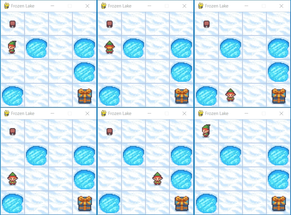
Frozen Lake
A Vision-based DQN method.
This project was completed by myself.

Deep Q-Network (DQN)
Q-learning is an algorithm that repeatedly adjusts Q Value to minimize the Bellman error.
\[Q(s_t,a_t) \leftarrow Q(s_t,a_t) + \alpha \underbrace{\left [ r(s,a) + \gamma \max_{a'} Q(s_{t+1},a') - Q(s_t,a_t) \right ]}_{\text{Bellman Error}}\]The Q-value function at state s and action a, is the expected cumulative reward from taking action a in state s and then following the policy:
\[Q(s,a) = \mathbb{E} \left [ \sum_{t \geq 0} \gamma^t r_t \right ]\]We learn these Q-values using the Q-learning algorithm.
The discount factor $\gamma$ is the weight for future rewards.
To percept is to see
extract_state_img
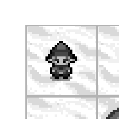
- This is the most important function in the whole program. It crops the current image into a smaller one so that the agent can see the environment around it. The reason why doing this is that the agent is truly expected to SEE the environment around it. The neural network for DQN in this program is based on convolutional neural networks.
def extract_state_img(env, state_idx, transforms):
    """
    Extracts the state image from the environment image.

    :param env: Frozenlake environment
    :param state_idx: Index of the state, range is 0-15
    :param transforms: Transform the image before return

    :return: Image of shape CxHxW
    """
    # Convert env rgb array to tensor
    env = torch.tensor(env.render('rgb_array'))
    block_size = env.shape[0] // 4

    # Extract state from given index
    env = env.permute(2, 0, 1)
    env = transforms(env)
    env = env.permute(1, 2, 0)

    start_idx = (state_idx // 4) * block_size
    end_idx = (state_idx % 4) * block_size
    state_img = env[start_idx:(start_idx + block_size + 2 * PADDING), end_idx:(end_idx + block_size + 2 * PADDING), :]

    state_img = state_img.permute(2, 0, 1).type(torch.float)
    return state_img


DQN Architecture
"""
DQN Architecture
"""
class DQN(nn.Module):
    def __init__(self, n_observations, n_actions):
        super(DQN, self).__init__()
        self.model = nn.Sequential(
            # 1, 104, 104
            nn.Conv2d(1, 32, kernel_size=8, stride=4),
            nn.ReLU(True),
            # 32, 25, 25
            nn.Conv2d(32, 64, kernel_size=5, stride=2),
            nn.ReLU(True),
            # 64, 11, 11
            nn.Conv2d(64, 64, kernel_size=3, stride=1),
            nn.ReLU(True),
            # 64, 9, 9
            nn.Flatten(),
            nn.Linear(9 * 9 * 64, 512),
            nn.ReLU(True),
            nn.Linear(512, n_actions),
        )

    def forward(self, x):
        return self.model(x)
This part mainly defines the model of DQN. Where input is a grayscale image and the outputs are actions.
DQN Agent
Q-learning is an algorithm that repeatedly adjusts Q Value to minimize the Bellman error. \(Q(s_t,a_t) \leftarrow Q(s_t,a_t) + \alpha \underbrace{\left [ r(s,a) + \gamma \max_{a'} Q(s_{t+1},a') - Q(s_t,a_t) \right ]}_{\text{Bellman Error}}\) As for the DQN, the loss function is comparing the difference between $Q(s_t, a_t)$ and $r(s,a) + \gamma \max_{a’}$, which is exactly the Bellman error. Specifically, the loss function for the neural network is the Smooth L1 Loss which is also knonw as the Huber Loss.
\[\left\{ \begin{aligned} 0.5 \cdot (x - y)^2,& \text{if} |x - y| < 1 \\ |x - y| - 0.5,& \text{otherwise} \end{aligned} \right.\]where:
- ( x ) represents the predicted value (e.g., predicted Q-value in the DQN).
- ( y ) represents the target value (e.g., target Q-value in the DQN). The Smooth L1 Loss behaves like the L1 loss (MAE) when the absolute difference between ( x ) and ( y ) is small (i.e., $( |x - y| < 1 )$), and it behaves like the L2 loss (MSE) when the absolute difference is large (i.e., $( |x - y| \geq 1 )$). This property makes the loss more robust to outliers and can lead to more stable training in some scenarios.
Soft copy
The copy operation of the parameter for target network is done by the formula shown as below: \(\theta ' \leftarrow \tau \cdot \theta + ( 1 - \tau) \cdot \theta '\) where $\theta$ is the parameter of the network.
Result
Visualised result of training process is shown as below:

Finally, the little agent had a high possibility of reaching the gift successfully.
For more information, see the work in my github repository!